

Excel is a very complete tool that offers you many possibilities, including the ability to create notes and grade sheets.
Excel is not only a very useful tool in the workplace, but not only for accountants and finance professionals, but also for teachers and educators, since they can carry out the administrative part of their work through this office tool. An example of this is when preparing the templates for student grades and grades to keep track and, in the end, determine who passes and who does not.
Fortunately, the latter is very easy to do, although it requires a fairly extensive process that you must follow rigorously . But if you need to make an Excel for notes and qualifications, then you’re in luck, because we will explain the step by step to carry it out. Although it will be necessary for you to learn some formulas and their functions , as they will be important later.
Excel is an office tool with a lot of potential and that can be very useful in various aspects of life. Therefore, it is recommended that, at least, you have basic knowledge in its handling . And a good way to do that is by learning the most important beginner formulas .
- First you must create the Excel structure for grades and grades
- You must fill in the fields with the information of the students
- Now, you must take the final grade point average of the students
- Use Excel’s conditional formula to determine passing and failing students.
First you must create the Excel structure for grades and grades

The first thing is to create the structure of the sheet for notes and grades in Excel
To begin, it is necessary to create the entire structure that the grades and grades sheet will have. In other words, you must design each of the fields and sections that, later, you will have to fill in with the information of the students.
But before that, logically, it is necessary that you have opened a new spreadsheet in Excel. It will be then that you can begin to design the fields , such as the names and surnames of the students, class periods, evaluations and the general average of each of these periods. At the end, you could include a Final Average section , which will be essential to know if, indeed, the student passes the course or not.
At this point, you are free to choose what design, colors, and data your grade sheet will include. Though you can look at the one we’ve created for some additional inspiration, should you need it.
You must fill in the fields with the information of the students
It is important that you fill in the fields with the information of the students, and their evaluation marks to calculate the academic average
After having created what will be the structure of the notes and qualifications sheet, it is necessary to proceed to fill in each of the blank fields . This means that you will have to manually type the names and surnames of each of the students, as well as take their ID into account.
But this is not all, since just below the evaluation fields, you will have to enter the grade that each student got . This includes research papers, written exams, and much more.
It is necessary that you repeat this process with all the students that you have in the enrollment, because from their individual grades in each evaluation, the mathematical operation will be carried out to calculate the general average of each academic period.
Depending on the number of lapses, you will have an overall average in each of these . But in order to get these results, you need to use the formula to get the averages.
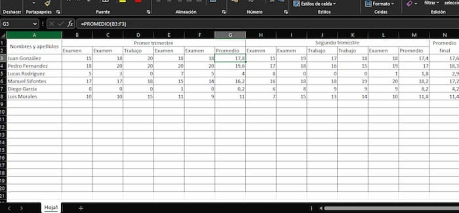
In Excel you have several ways to obtain the average of several quantities. The first of these is using the Insert function button that is located just above the cells and that displays a series of mathematical operations . Here you can click on the Average option and select all the marks that the student obtained in the evaluations. At the end, click OK and the mathematical calculation will be performed.
If you prefer to do it faster, then you should go to the cell corresponding to the student’s average and type the formula =AVERAGE(first grade cell:last grade cell) and press Enter . According to the example we have prepared, it would remain for the average of the student’s first quarter: =AVERAGE(B3:BF) .
You must repeat this with all the students and this can be done in two ways. The first is through the manual method of re-entering the formula in all the average cells, changing the data for each student . Or you can do it like a professional and click on the cell where you have made the first average calculation and you will see that it will show a kind of cross in the lower right part. You simply have to click on this symbol and extend it to the cells below.
What it will do is repeat the mathematical formula of the average, but with the respective data of the following students. This will save you time and look like a professional.
Now, you must take the final grade point average of the students
In order to obtain the final average of the students’ grades, it is necessary to have all the averages of the academic periods.
If the educational institution where you work uses a system of two quarters, one semester or some other, then you will obtain several averages that the students have achieved in the different educational periods.
And now it is time to use these averages of the periods to obtain the final period of notes , which will be essential to determine if the students have passed the course or not. Fortunately, this is the same or easier to do.
Again, to get the final grade point average , you can use two methods. The first is to click on the Final Average cell and then click on the Insert Function button and choose Average . After this, a floating window will open where you must enter the values that will be taken into account.
This is when you must hold down the CTRL key and click on the result of the first average and, without releasing said key, you click on the second average . And click OK . You can select more cells, depending on the number of averages you are working with.
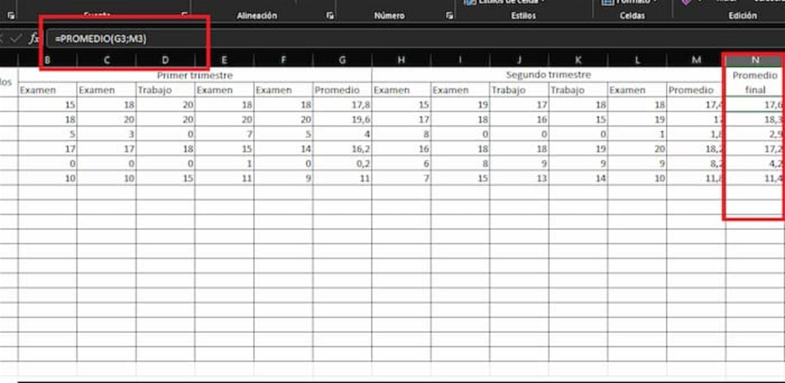
The quickest and easiest way to calculate the final grade point average is to click in the corresponding cell, then type the formula =AVERAGE(first average; second average) and press Enter . This will perform the mathematical calculation and show you the result.
According to the example we have designed, the formula would be =AVERAGE(G3,M3) . Then you must repeat this same procedure for the rest of the final averages of the students.
Use Excel’s conditional formula to determine passing and failing students
With this logical formula you will be able to determine if the students have passed or failed the course
Finally, to finalize this Excel for grades and grades, it is time to determine which students pass the course and which fail . For this, it will be necessary to have all the notes already entered in the template and to have calculated all the averages.
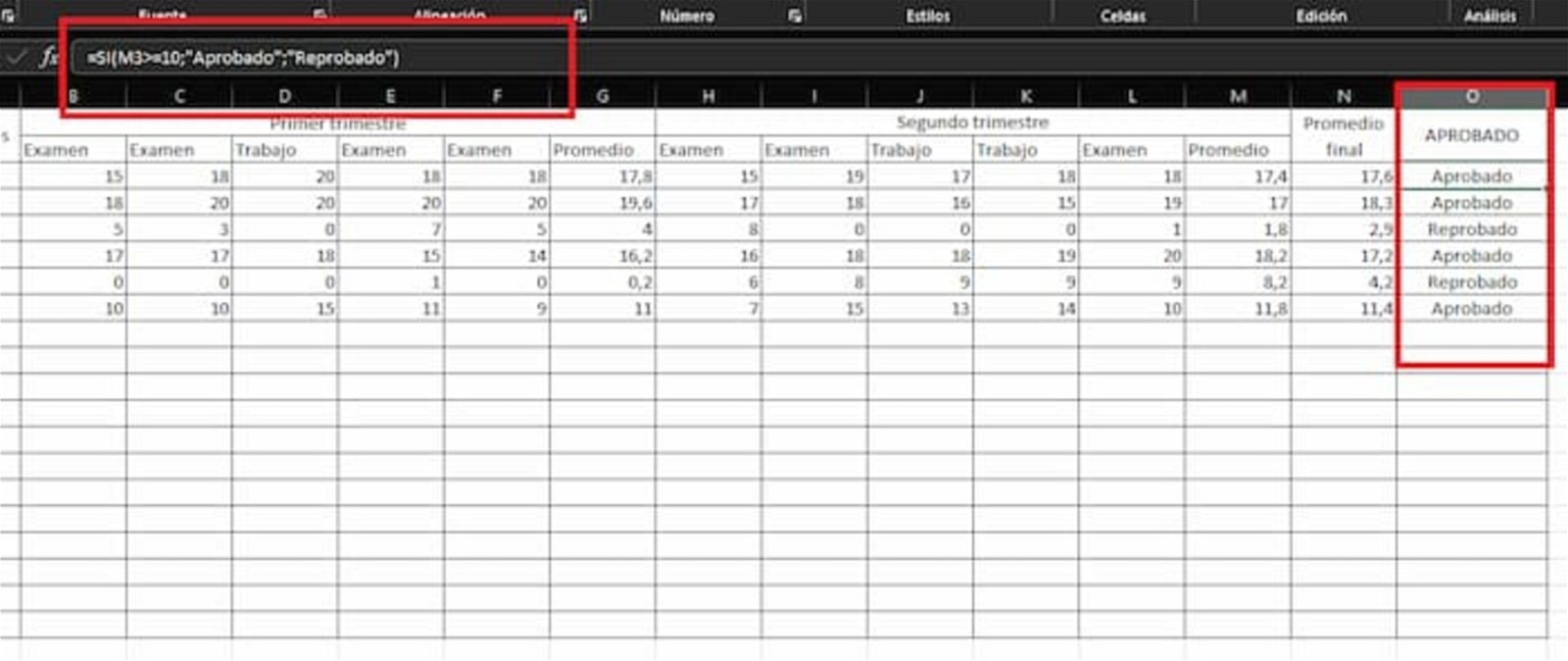
For our example, we have taken an institution in which, to pass a course, it is necessary to have a minimum of 10 points and a maximum of 20 points . That is why all students who, in their final average, have obtained more than 10 points will have passed, while those with a lower score will fail.
It is important to take into account that, to determine this result , it will be necessary to use the formula of the logical IF conditional and that would be: =SI(final average cell>=10;”Approved”;”Failed”) . In our example, it would be =IF(M3>=10;”Approved”;”Failed”) .
Pressing the Enter button will make this determination and will write Approved or Failed , depending on the final average of each student. And you must repeat this process with each one. Although, to speed things up, you can extend the application of the formula as we have explained before.


